import math
import matplotlib.pyplot as plt
gamma = 1.4
num_value = 50
#engine kinematics function
def engine_parameters(bore,stroke,con_rod,cr,start_crank,end_crank,v_s,v_c):
a = stroke/2
R = con_rod/a
sc=math.radians(start_crank)
ec=math.radians(end_crank)
dtheta = (ec-sc)/(num_value-1)
V = []
for i in range(0,num_value):
theta = sc+ i*dtheta
term1 = 0.5*(cr-1)
term2 = R+1-math.cos(theta)
term3 = pow(R,2) - pow(math.sin(theta),2)
term3 = pow(term3,0.5)
V.append((1+term1*(term2-term3))*v_c)
return V
#graph function
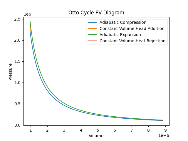
def graph_plot():
plt.figure(1)
plt.plot(V_compression,P_compression,label='Adiabatic Compression')
plt.plot([v2,v3],[p2,p3],label='Constant Volume Head Addition')
plt.plot(V_expansion,P_expansion,label='Adiabatic Expansion')
plt.plot([v4,v1],[p4,p1],label='Constant Volume Heat Rejection')
plt.xlabel('Volume')
plt.ylabel('Pressure')
plt.legend()
plt.title('Otto Cycle PV Diagram')
plt.savefig('otto_cycle_pv_diagram.png')
plt.show()
#Define Inputs
p1 = float(input("Type the value for P1: (Pa) \t"))
t1 = float(input("Type the value for T1: (K) \t"))
t3 = float(input("Type the value for T3: (K) \t"))
bore = float(input("Type the value for bore diameter: (m) \t"))
stroke = float(input("Type the value for length of stroke: (m)\t"))
con_rod = float(input("Type the value for length of connecting rod:(m) \t"))
cr = int(input("Type the value for Compression Ratio:\t"))
# Calculate Volumes
v_s = (math.pi/4)*pow(bore,2)*stroke
v_c=v_s/(cr-1)
v1=v_s+v_c
v2=v_c
#calculate state point 2
p2 = p1*pow(v1,gamma)/pow(v2,gamma)
rhs =p1 *v1/t1
t2 =p2*v2/rhs
#compression process
V_compression =engine_parameters(bore,stroke,con_rod,cr,180,0,v_s,v_c)
constant =p1*pow(v1,gamma)
P_compression=[constant/pow(v,gamma) for v in V_compression]
#calculate state point 3
v3=v2
rhs=p2*v2/t2
p3=rhs*t3/v3
expansion process
V_expansion=engine_parameters(bore,stroke,con_rod,cr,0,180,v_s,v_c)
constant =p3*pow(v3,gamma)
P_expansion =[constant/pow(v,gamma) for v in V_expansion]
#state point 4
v4 = v1
p4 =p3*pow(v3,gamma)/pow(v4,gamma)
rhs=p3*v3/t3
t4=p4*v4/rhs
eff = 1 - (1 / pow(cr, (gamma - 1)))
eff_percent = eff * 100
print(f'Thermal Efficiency: {eff_percent:.2f}%')
graph_plot()